
Plotting#
Every data object has a plot namespace with the plotting functions
(PlotNamespace), e.g. d.plot.plot_pupil();
dir(d.plot) lists them. Pupil plots need pupil data and gaze plots need
gaze data; they raise an error if the data are missing. Gaze plots draw the
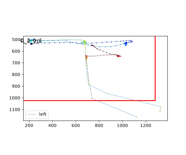
screen as it is seen: pixel y increases downward. All plots use
matplotlib, so they can be adjusted and saved as usual. Most
functions take eyes=, variables=, plot_range= and units=
arguments. units= is the unit of the time axis and of plain numbers
in plot_range (and interv of the *_segments plots):
plot_range=(0, 20), units="sec" plots the first 20 seconds. Values
with units are converted, e.g., plot_range=(0, 20) * u.sec. In all
plots that have it, plot_range is the first argument, so it can be
given without its name: d.plot.plot_pupil((0, 20) * u.sec).
The examples on this page use the short example dataset with detected blinks:
import pypillometry as pp
from pypillometry import u
import matplotlib.pyplot as plt

d = pp.get_example_data("rlmw_002_short")
d.pupil.blinks_detect()
Each function’s API documentation has another example.
Figures and axes#
All plotting functions follow one of three conventions, depending on how many panels and figures they draw:
One panel (e.g.,
plot_pupil(),plot_masked(),plot_scanpath(),Events.plot(),Intervals.plot(), the plots of the segments and of ROIs): the plot is drawn onax=(default: the current axes), and the axes are returned. Several plots can be combined in one figure this way:fig, axs = plt.subplots(2, 1, figsize=(10, 6)) d.plot.plot_pupil(plot_range=(0, 20) * u.sec, ax=axs[0]) d.plot.plot_pupil(plot_range=(20, 40) * u.sec, ax=axs[1])
Several panels in one figure (
plot_timeseries(),plot_heatmap(),plot_calibration(), …): the function makes a new figure of sizefigsize=and returns it.axes=(one axes per panel) draws on existing axes instead, e.g.,fig.axesof an earlier call to overlay two datasets.Several figures (
plot_blinks(),plot_intervals()and the*_segmentsplots): a list of figures of sizefigsize=is returned; withpdf_file=, they are also written to a multi-page PDF file (and closed).
All of them take title=, and the one-panel plots pass further
arguments to matplotlib (e.g., color="red"; see the API documentation
of each function). In a notebook, end a line with a plotting function with
; (or assign the result) to hide the returned object.
Time series#
Make a plot of the pupil data using matplotlib. |
|
Plot a part of the EyeData. |
|
Plot masked intervals for specified eyes and variables. |
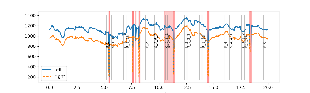
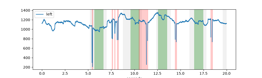
plot_pupil() shows the pupil size of all eyes in one
plot, with blinks (red) and events (grey lines):
fig, ax = plt.subplots(figsize=(10, 3))
d.plot.plot_pupil(plot_range=(0, 20) * u.sec, ax=ax)
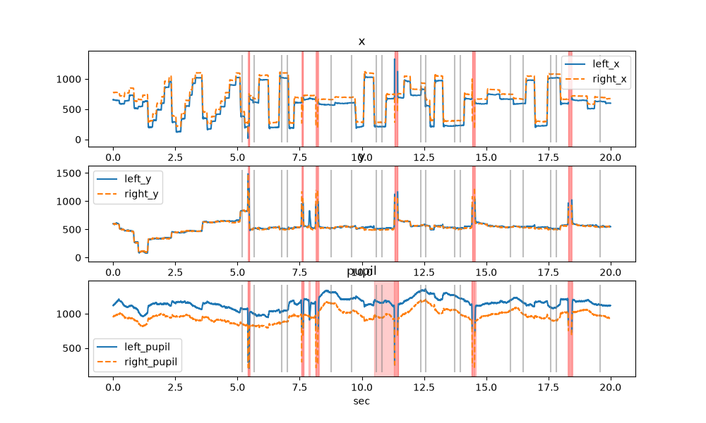
plot_timeseries() plots each variable (here: gaze and
pupil) in its own panel:
fig = d.plot.plot_timeseries(plot_range=(0, 20) * u.sec, units="sec",
                             figsize=(10, 6))
To save a plot, use matplotlib as usual, e.g.
fig.savefig("pupil.pdf").
Long recordings#
Plotting a whole recording at once hides the details. These functions split
it into many small plots (one figure each), optionally written to a
multi-page PDF file with pdf_file=. For interactive browsing, the
viewer is usually faster.
Plot the whole dataset chunked up into segments (usually to a PDF file). |
|
Plot the whole dataset chunked up into segments (usually to a PDF file). |
Blinks and intervals#
Plot detected blinks in separate subplots. |
|
Plotting data around intervals. |
|
Plot intervals as horizontal lines on a timeline. |
|
Plot events as points on a time axis. |
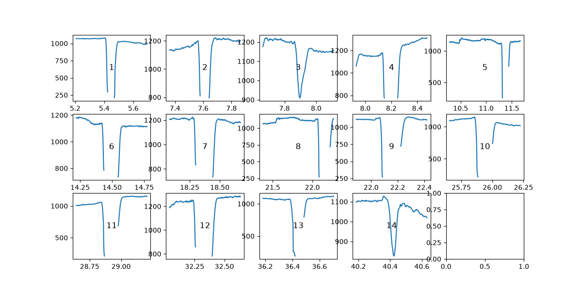
plot_blinks() draws one small plot per blink, e.g., to
check blink detection and interpolation:
figs = d.plot.plot_blinks(eyes="left", nrow=3, ncol=5, figsize=(12, 6),
                          units="sec")
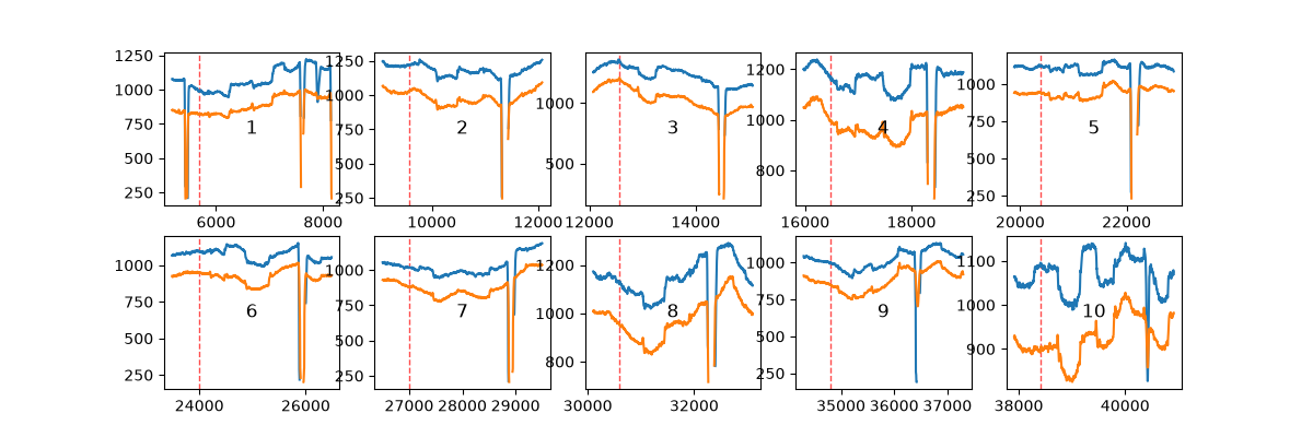
plot_intervals() does the same for any
Intervals, here the three seconds around each stimulus:
epochs = d.get_epochs("S_", (-500, 2500) * u.ms)
figs = d.plot.plot_intervals(epochs, variables="pupil", nrow=2, ncol=5,
                             figsize=(12, 4))
The plots with a time axis (plot_pupil(),
plot_timeseries(), plot_masked()
and the *_segments plots) shade Intervals or Epochs
with highlight=. They are converted to the units of the time axis. A
list of them gets one color each from highlight_color=:
trials = d.get_intervals(start="F_", end="R_")
stim = d.get_epochs("S_", (0, 1000) * u.ms)
fig, ax = plt.subplots(figsize=(10, 3))
d.plot.plot_pupil(eyes="left", plot_range=(0, 20) * u.sec, ax=ax,
                  show_events=False, highlight=[trials, stim],
                  highlight_color=["lightgrey", "green"])
Event-related pupil dilation#
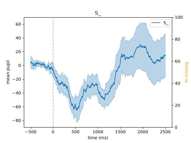
The segments returned by get_segments() have their
own plots that show the mean (with its standard error) and the
percentage of missing data: seg.pupil.plot() for the pupil (the
event-related pupil dilation), seg.gaze.plot_roi() for the share of
trials in which the gaze is in a region of interest, and seg.plot()
for any channel (see Events, intervals and segments):
d.pupil.blinks_interpolate()
epochs = d.get_epochs("S_", (-500, 2500) * u.ms)
erpd = d.get_segments(epochs, "left_pupil").pupil.baseline_correct((-500, 0))
erpd.pupil.plot()
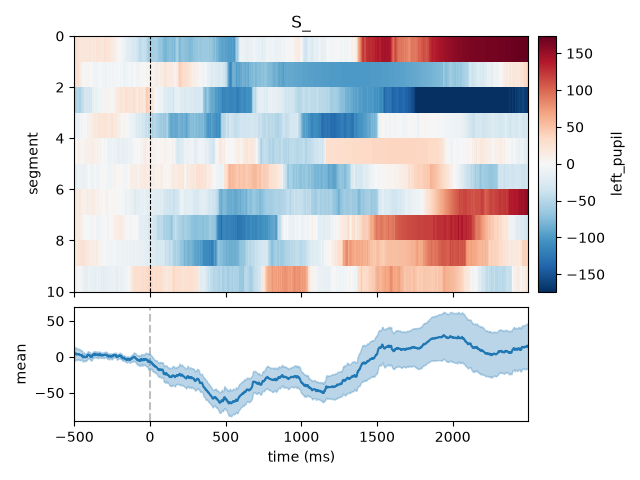
plot_carpet() shows all segments of a channel
instead of their mean: one row per trial, the value as color (a “carpet
plot”). It shows how the response varies between trials, e.g., trials with
artifacts or a change over the session; sort_by= orders the rows by
a property of the trials (e.g., a metadata column such as the reaction
time), and show_mean=True adds the mean below the image:
erpd.plot_carpet(show_mean=True)
Plot the event-related pupil dilation: mean and error ribbon of the pupil channels over time. |
|
Plot the share of trials in which the gaze is in a region of interest over time (fixation curve), with an error ribbon. |
|
Plot mean and error ribbon over time, one line per channel. |
|
Plot all segments of one channel as an image ("carpet plot"). |
Gaze#
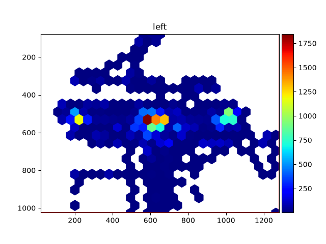
Plot EyeData as a heatmap. |
|
Plot EyeData as a scanpath. |
|
Plot spatial calibration data for one or more eyes in subplots. |
fig = d.plot.plot_heatmap(eyes="left")

fig, ax = plt.subplots(figsize=(6, 5))
d.plot.plot_scanpath(plot_range=(10, 12) * u.sec, eyes="left", ax=ax)
plot_calibration() shows the calibration and validation
results of the eye tracker (see Spatial calibration).
Regions of interest can be drawn on top of heatmaps and scan paths (see
Experimental setup and regions of interest).
Comparing versions of the data#
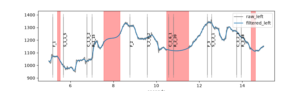
To compare, e.g., raw and filtered data, plot both into the same axes
(ax= for one-panel plots, axes=fig.axes for
plot_timeseries()) and give each a label_prefix
and a style:
filtered = d | pp.pupil.lowpass_filter(cutoff=4)

fig, ax = plt.subplots(figsize=(10, 3))
d.plot.plot_pupil(eyes="left", plot_range=(5, 15) * u.sec, ax=ax,
                  label_prefix="raw", style={"color": "grey"})
filtered.plot.plot_pupil(eyes="left", plot_range=(5, 15) * u.sec, ax=ax,
                         label_prefix="filtered")
See the tutorial Plotting pupillometric data for exploration for more examples.