Plotting (`d.plot`)#

Each data object has a plot namespace with the plotting functions, e.g. d.plot.plot_pupil() (see Plotting). You do not create it yourself. The plots draw into the current matplotlib figure (or create one).

Time series#

`plot.PlotNamespace.plot_pupil`	Make a plot of the pupil data using matplotlib.
`plot.PlotNamespace.plot_timeseries`	Plot a part of the EyeData.
`plot.PlotNamespace.plot_pupil_segments`	Plot the whole dataset chunked up into segments (usually to a PDF file).
`plot.PlotNamespace.plot_timeseries_segments`	Plot the whole dataset chunked up into segments (usually to a PDF file).

Blinks, masks and intervals#

`plot.PlotNamespace.plot_blinks`	Plot detected blinks in separate subplots.
`plot.PlotNamespace.plot_masked`	Plot masked intervals for specified eyes and variables.
`plot.PlotNamespace.plot_intervals`	Plotting data around intervals.

Gaze#

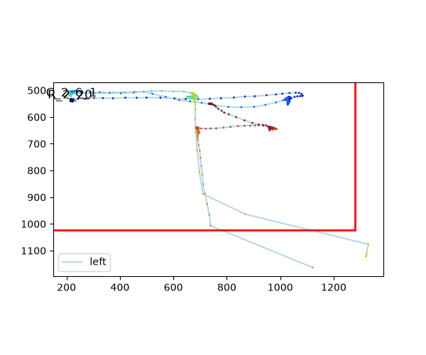
`plot.PlotNamespace.plot_heatmap`	Plot EyeData as a heatmap.
`plot.PlotNamespace.plot_scanpath`	Plot EyeData as a scanpath.
`plot.PlotNamespace.plot_calibration`	Plot spatial calibration data for one or more eyes in subplots.

Experimental setup and foreshortening#

`plot.PlotNamespace.plot_experimental_setup`	Plot visualization of eye-tracking experimental setup geometry.
`plot.PlotNamespace.plot_pupil_foreshortening_error_surface`	Plot a heatmap showing average pupil size across x/y gaze positions.

The segmented data have their own plots (SegmentedEyeData.plot(), seg.pupil.plot(), seg.gaze.plot_roi()).

All plots#

class pypillometry.plot.PlotNamespace(data=None)[source]#

Plotting methods of an EyeData object, used as d.plot (e.g., d.plot.plot_timeseries()).

Like d.pupil and d.gaze, it is a view on the data object with no state of its own (see Namespace). It combines the generic plots, the pupil plots and the gaze plots, which are written in separate modules. Plots that need channels the object does not have raise a ValueError.

plot_blinks(eyes=[], variables='pupil', pdf_file=None, nrow=5, ncol=3, figsize=(10, 10), pre_blink=200, post_blink=200, units='sec', show_index=True)#

Plot detected blinks in separate subplots.

Parameters:

eyes (str | list) – Eyes to plot
variables (str | list) – Variables to plot
pdf_file (str | None) – Save to PDF file if provided
nrow (int) – Number of rows per figure
ncol (int) – Number of columns per figure
figsize (tuple) – Figure size (width, height)
pre_blink (float) – Time before blink to include (in ms)
post_blink (float) – Time after blink to include (in ms)
units (str) – Display units for time axis; default “sec”
show_index (bool) – Show blink index numbers

Return type:

list

Returns:

one figure per nrow x ncol blinks (also returned when pdf_file is given; the figures are then closed)

Raises:

ValueError – if the object has no data for variables

Examples

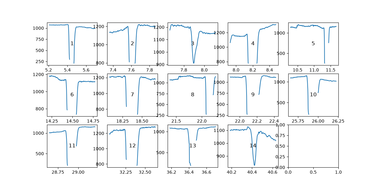
Check the detected blinks of the left eye (the numbers are the blink indices):

>>> import pypillometry as pp
>>> from pypillometry import u
>>> import matplotlib.pyplot as plt
>>> d = pp.get_example_data("rlmw_002_short")
>>> d = d.pupil.blinks_detect()
>>> figs = d.plot.plot_blinks(eyes="left", nrow=3, ncol=5, figsize=(12, 6),
...                           units="sec")

plot_calibration(eyes=None, show_surface=True, interpolation='rbf', title=None, axes=None, figsize=None)#

Plot spatial calibration data for one or more eyes in subplots.

Plots each eye in a separate subplot with the plot() method of its SpatialCalibration object: calibration accuracy with target points (black X), measured points (dark blue +), and optional interpolated error surface.

Parameters:

eyes (Union[str, list, None]) – Which eye(s) to plot. If None or empty list, plots all available eyes. Can be a single eye name (e.g., ‘left’) or list of eye names (e.g., [‘left’, ‘right’]).
show_surface (bool) – If True, show interpolated error surface as background. If False, show only the calibration points.
interpolation (str) – Interpolation method for surface (only used if show_surface=True). Options: ‘rbf’, ‘linear’, ‘cubic’, ‘nearest’
title (str) – title of the figure
axes (list of matplotlib.axes.Axes, optional) – axes to plot on, one per eye; default: a new figure (one subplot per eye, side by side)
figsize (tuple) – size of the new figure; default: 10 x 8 inches per eye

Return type:

matplotlib.figure.Figure

Returns:

the figure of the plot

Raises:

ValueError – If no calibration data is available, or if axes does not contain one axes per eye

Examples

>>> import pypillometry as pp
>>> data = pp.EyeData.from_eyelink('data.edf')
>>> # Plot all eyes with surface
>>> fig = data.plot.plot_calibration()
>>> 
>>> # Plot only left eye without surface
>>> fig = data.plot.plot_calibration(eyes='left', show_surface=False)
>>> 
>>> # Plot specific eyes
>>> fig = data.plot.plot_calibration(eyes=['left', 'right'])

plot_experimental_setup(theta=None, phi=None, calibration=None, show_gaze_samples=True, n_gaze_samples=9, viewing_angle=None, projection='2d', title=None, axes=None, figsize=None)#

Plot visualization of eye-tracking experimental setup geometry.

Shows the spatial relationship between eye, camera, and screen using the experimental parameters stored in the EyeData object. Delegates to ExperimentalSetup.plot().

Parameters:

theta (Optional[float]) – Camera polar angle; a float is interpreted as radians, a string can carry units (e.g., “20 deg”). If None, uses calibration’s theta (if calibration is given), else setup’s theta.
phi (Optional[float]) – Camera azimuthal angle; a float is interpreted as radians, a string can carry units (e.g., “-90 deg”). If None, uses calibration’s phi (if calibration is given), else setup’s phi.
calibration (ForeshorteningCalibration, optional) – Fitted calibration object containing theta and phi.
show_gaze_samples (bool) – Show sample gaze vectors to screen positions
n_gaze_samples (int) – Number of sample gaze positions
viewing_angle (tuple) – Viewing angle for 3D projection (elev, azim) or (elev, azim, roll). Plain numbers are in degrees (as in matplotlib’s view_init); strings with units (e.g., ("30 deg", "-60 deg")) are parsed.
projection (str) – ‘2d’ for three orthogonal views, ‘3d’ for interactive 3D view
title (str) – title of the figure; default: the camera angles
axes (matplotlib Axes or list of Axes, optional) – axes to plot on: three axes (front, top, side view) for ‘2d’, one 3D axes for ‘3d’; default: a new figure
figsize (tuple) – size of the new figure

Return type:

matplotlib.figure.Figure

Returns:

the figure (fig.axes are the axes of the views)

Raises:

ValueError – if the data object has no experimental_setup

Examples

Camera geometry from the experimental setup:

>>> import pypillometry as pp
>>> from pypillometry import u
>>> import matplotlib.pyplot as plt
>>> d = pp.get_example_data("rlmw_002_short")
>>> d = d.set_experimental_setup(camera_spherical=("20 deg", "-90 deg", "70 cm"))
>>> fig = d.plot.plot_experimental_setup()

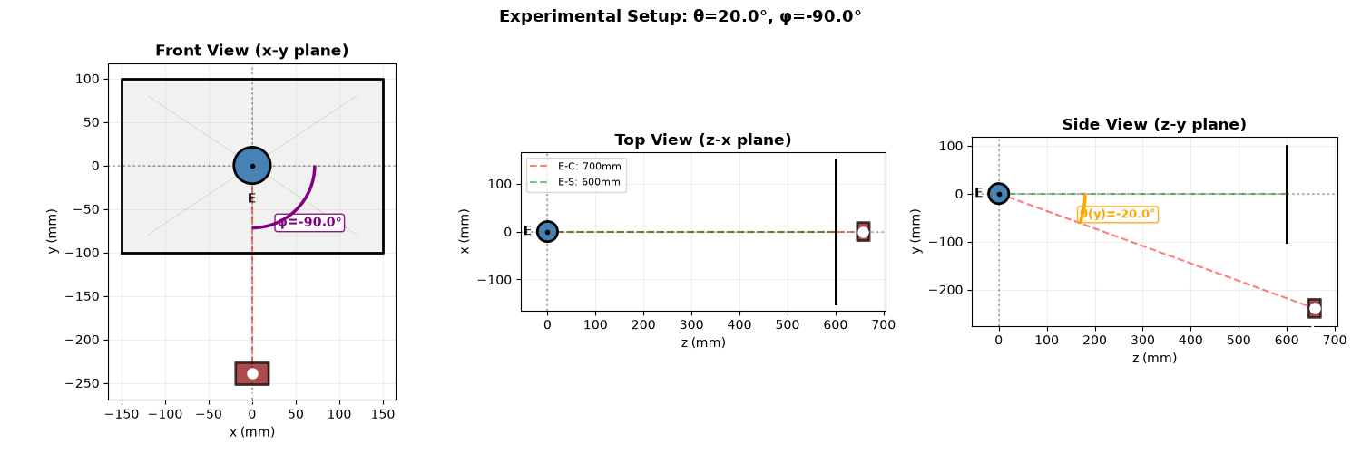
To show fitted angles, pass the result of d.pupil.fit_foreshortening() as calibration=, or set theta/phi directly.

plot_heatmap(plot_range=(-inf, inf), eyes=[], show_screen=True, show_masked=False, rois=None, roi_style={}, units='sec', cmap='jet', gridsize=30, min_samples=1, smooth=None, limits=None, title=None, axes=None, figsize=None)#

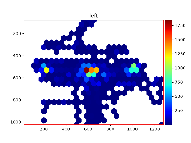
Plot EyeData as a heatmap. Typically used for a large amount of data to spot the most frequent locations. To plot a scanpath, use plot_scanpath() instead. Each eye is plotted in a separate subplot; the colorbar shows the number of samples per bin. The y-axis points down (screen pixel coordinates, as in plot_calibration()).

Parameters:

plot_range (tuple) – The time range to plot (plain numbers are in units, or with units, e.g. (3, 5) * u.min). Default is (-np.inf, +np.inf), i.e. all data.
eyes (list) – The eyes to plot. Default is [], which means all available data (“left”, “right”, average, regression, …)
show_screen (bool) – Whether to plot the screen limits (if an experimental setup is available). Default is True.
show_masked (bool) – Whether to plot the masked data (because of blinks, artifacts, …; default mask policy). Default is False.
rois (List[ROI]) – List of ROIs (ROI) to plot. Default is None.
roi_style (dict) –
Style for the ROIs, passed as keyword arguments to the ROIs’ plot() method. Default is {} (ROI defaults). Example:
```
{
    "facecolor": "red",
    "edgecolor": "black",
    "linewidth": 2,
    "alpha": 0.5
}
```
units (str) – The units of plain numbers in plot_range and of messages (“ms”, “sec”, “min”, “h”). Default is “sec”.
cmap (str) – The colormap to use. Default is “jet”.
gridsize (int | str) – The gridsize for the hexbin plot or histogram. If “auto”, the square root of the number of samples in plot_range is used. Default is 30.
min_samples (Optional[int]) – Minimum number of samples required in a bin to display it. Bins with fewer samples will not be shown. If None, automatically calculates a threshold at the 10th percentile of bin counts. Default is 1.
smooth (Optional[float]) – If provided, applies Gaussian smoothing to the binned histogram. The value is the sigma of the Gaussian kernel in bin units (e.g., smooth=1 applies minimal smoothing with a 1-bin sigma, smooth=2 applies more smoothing). When smooth is provided, uses a rectangular grid instead of hexbin.
limits (Optional[Tuple[float, float, float, float]]) – Axis limits as (xmin, xmax, ymin, ymax). If not provided, uses screen limits when available (and data falls within), otherwise uses data extent.
title (str) – title of the figure
axes (list of matplotlib.axes.Axes, optional) – axes to plot on, one per eye; default: a new figure (one subplot per eye, side by side)
figsize (tuple) – size of the new figure

Return type:

matplotlib.figure.Figure

Returns:

the figure of the plot (fig.axes also contains the colorbars)

Raises:

ValueError – if plot_range does not overlap with the data

Examples

>>> import pypillometry as pp
>>> from pypillometry import u
>>> import matplotlib.pyplot as plt
>>> d = pp.get_example_data("rlmw_002_short")
>>> fig = d.plot.plot_heatmap(eyes="left")

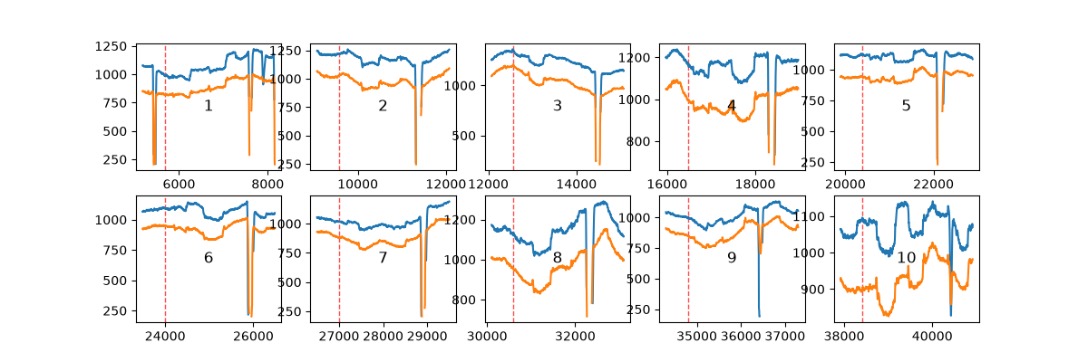
plot_intervals(intervals, eyes=[], variables=[], pdf_file=None, nrow=5, ncol=3, figsize=(10, 10), show_mask=False, show_index=True)#

Plotting data around intervals.

Intervals can be extracted with get_epochs() or get_intervals(). Each interval gets a separate subplot. The data is plotted for each eye and variable in different colors. The x-axis is plotted in the units of the Intervals object. If the intervals contain event onsets, these are marked by a dashed red line.

Parameters:

intervals (Intervals) – the intervals to plot (e.g., from get_epochs()); Epochs are plotted in ms, with a line at each event onset
eyes (str | list) – eyes to plot; if empty, all available eyes are plotted
variables (str | list) – variables to plot; if empty, all available variables are plotted
pdf_file (Optional[str]) – if the name of a file is given, the figures are saved into a multi-page PDF file (missing directories are created)
nrow (int) – number of rows for the subplots for the intervals
ncol (int) – number of columns for the subplots for the intervals
figsize (Tuple[int, int]) – size (width, height) of each figure in inches
show_mask (bool) – shade samples masked (default mask policy) in any of the plotted eyes/variables
show_index (bool) – plot a number with the interval’s index (e.g., for identifying abnormal blinks)

Return type:

list of matplotlib.figure.Figure

Returns:

one figure per nrow x ncol intervals (also returned when pdf_file is given; the figures are then closed)

Raises:

TypeError – if intervals is not an Intervals or Epochs object

Examples

The pupil around each stimulus, one panel per interval:

>>> import pypillometry as pp
>>> from pypillometry import u
>>> import matplotlib.pyplot as plt
>>> d = pp.get_example_data("rlmw_002_short")
>>> epochs = d.get_epochs("S_", (-500, 2500) * u.ms)
>>> figs = d.plot.plot_intervals(epochs, variables="pupil", nrow=2, ncol=5,
...                              figsize=(12, 4))

plot_masked(eyes=[], variables=[], units='sec', merge=False, show_labels=True, show_events=False, policy='default', highlight=None, highlight_color='lightblue', title=None, ax=None, **kwargs)#

Plot masked intervals for specified eyes and variables.

Visualizes masked data segments as horizontal lines on a timeline, similar to Intervals.plot(). Each interval is shown at a different y-level. When plotting multiple eyes/variables without merging, each is shown in a different color with slight y-offsets for clarity.

Parameters:

eyes (str | list) – Eye(s) to plot masks for. If empty, uses all available eyes.
variables (str | list) – Variable(s) to plot masks for. If empty, uses all available variables.
units (str) – Time units for x-axis: “ms”, “sec”, “min”, “h”, or “samples” for sample indices. Default is “sec”.
merge (bool) – If True, merge all masks into a single set of intervals for plotting. If False, plot each eye/variable separately with different colors. Default is False.
show_labels (bool) – Whether to show a legend of the eyes/variables and a title. Default is True.
show_events (bool) – Whether to show vertical grey stripes at event positions. Default is False.
policy (str, MaskPolicy or list of str) – mask policy that decides which samples are masked (see mask_as_intervals()); e.g., "strict" also shows the interpolated samples, ["interpolated"] only those. Default "default".
highlight (Intervals, Epochs or list of them, optional) – periods to shade in the background (e.g., trials from get_intervals()), converted to the units of the time axis
highlight_color (color or list of colors, optional) – color of the shading: one for all or one per element of highlight; default “lightblue”
title (str) – title of the plot; default: “Masked Intervals” (if show_labels)
ax (matplotlib.axes.Axes, optional) – axes to plot on; default: the current axes
**kwargs (dict) – Additional keyword arguments passed to matplotlib.axes.Axes.plot()

Return type:

matplotlib.axes.Axes

Returns:

the axes of the plot

Examples

One line per masked interval (here: detected blinks) and eye:

>>> import pypillometry as pp
>>> from pypillometry import u
>>> import matplotlib.pyplot as plt
>>> d = pp.get_example_data("rlmw_002_short")
>>> d = d.pupil.blinks_detect()
>>> fig, ax = plt.subplots(figsize=(8, 4))
>>> ax = d.plot.plot_masked(variables="pupil", units="sec", ax=ax)

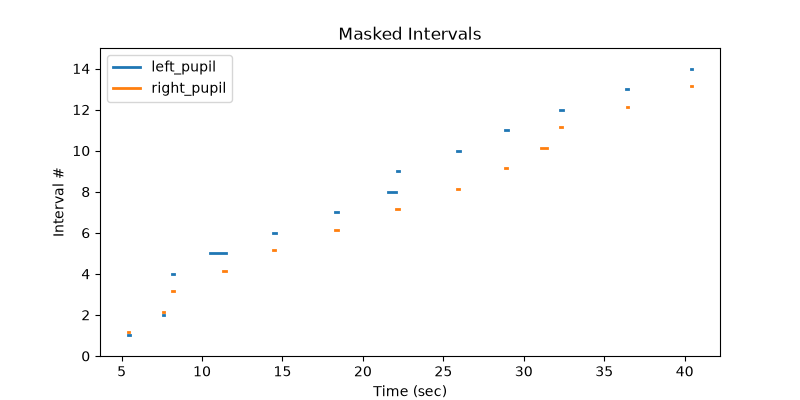
With merge=True, the masks of all eyes and variables are combined; show_events=True adds the event markers.

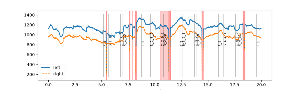
plot_pupil(plot_range=(-inf, inf), eyes=[], show_events=True, show_blinks=True, units='sec', label_prefix='', style=None, highlight=None, highlight_color='lightblue', title=None, ax=None, **kwargs)#

Make a plot of the pupil data using matplotlib.

Has pupil-specific options which makes it different from plot_timeseries(). All eyes are plotted into one axes (ax, or the current axes).

Parameters:

plot_range (Tuple[float, float]) – plot from start to end (plain numbers are in units, or with units, e.g. (3, 5) * u.min)
eyes (str | list) – eye(s) to plot; if empty, all eyes with pupil data are plotted
show_events (bool) – plot events as vertical lines with labels
show_blinks (bool) – highlight masked or interpolated regions of the pupil data (e.g., detected blinks; the "strict" mask policy) with a red background
units (str) – units of the time axis: one of “sec”=seconds (default), “ms”=millisec, “min”=minutes, “h”=hours
label_prefix (str) – Prefix to add to labels in the legend. Useful for overlaying multiple datasets. Default is “” (no prefix).
style (dict) –
Styling for plotted lines. Can be:
- Single dict: Applied to all eyes with automatic differentiation (e.g., {‘color’: ‘red’})
- Dict of dicts: Per-eye styling (e.g., {‘left’: {‘linestyle’: ‘-‘}, ‘right’: {‘linestyle’: ‘–‘}})
Default is None (uses matplotlib defaults with automatic per-eye colors and linestyles).
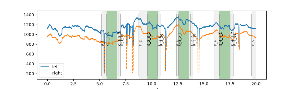
highlight (Intervals, Epochs or list of them, optional) – periods to shade in the background (e.g., trials from get_intervals()), converted to the units of the time axis
highlight_color (color or list of colors, optional) – color of the shading: one for all or one per element of highlight; default “lightblue”
title (str) – title of the plot
ax (matplotlib.axes.Axes, optional) – axes to plot on; default: the current axes
**kwargs – passed to matplotlib.axes.Axes.plot() for all eyes (after style)

Return type:

matplotlib.axes.Axes

Returns:

the axes of the plot

Raises:

ValueError – if plot_range does not overlap with the data

Examples

Detected blinks are shaded in red, events are shown as vertical lines:

>>> import pypillometry as pp
>>> from pypillometry import u
>>> import matplotlib.pyplot as plt
>>> d = pp.get_example_data("rlmw_002_short")
>>> d = d.pupil.blinks_detect()
>>> fig, ax = plt.subplots(figsize=(10, 3))
>>> ax = d.plot.plot_pupil(plot_range=(0, 20) * u.sec, ax=ax)

Shade the trials (feedback to response) and the first second after each stimulus in different colors:

>>> import pypillometry as pp
>>> from pypillometry import u
>>> import matplotlib.pyplot as plt
>>> d = pp.get_example_data("rlmw_002_short")
>>> trials = d.get_intervals(start="F_", end="R_")
>>> stim = d.get_epochs("S_", (0, 1000) * u.ms)
>>> fig, ax = plt.subplots(figsize=(10, 3))
>>> ax = d.plot.plot_pupil(plot_range=(0, 20) * u.sec, show_blinks=False,
...                        highlight=[trials, stim],
...                        highlight_color=["lightgrey", "green"], ax=ax)

plot_pupil_foreshortening_error_surface(plot_range=(-inf, inf), eyes=[], units='sec', show_screen=True, cmap='jet', gridsize=30, vmin=None, vmax=None, min_samples=None, smooth=None, limits=None, title=None, axes=None, figsize=None)#

Plot a heatmap showing average pupil size across x/y gaze positions.

This visualizes how pupil size varies across different gaze positions, which can reveal foreshortening effects (pupils appear smaller when looking away from the camera) or other spatial artifacts. Each eye is plotted in a separate subplot.

Parameters:

plot_range (tuple) – The time range to include in the analysis (plain numbers are in units, or with units, e.g. (3, 5) * u.min). Default is (-np.inf, +np.inf), i.e. all data.
eyes (Union[str, List[str]]) – Which eye(s) to plot: “left”, “right”, “average”, or a list of these. Default is [] which plots all eyes with pupil and gaze data; a requested eye without them raises a KeyError.
units (str) – Time units of the plot. Default is “sec”.
show_screen (bool) – Whether to plot the screen limits. Default is True.
cmap (str) – Colormap to use. Default is “jet”.
gridsize (int) – Number of bins in each direction. Default is 30.
vmin (Optional[float]) – Minimum value for color scale. If None, uses data minimum.
vmax (Optional[float]) – Maximum value for color scale. If None, uses data maximum.
min_samples (Optional[int]) – Minimum number of samples required in a bin to display it. Bins with fewer samples will not be shown. If None (default), automatically calculates a threshold at the 10th percentile of bin counts, effectively displaying only the top 90% of bins by sample count.
smooth (Optional[float]) – If provided, applies Gaussian smoothing to the binned surface. The value is the sigma of the Gaussian kernel in bin units (e.g., smooth=1 applies minimal smoothing with a 1-bin sigma, smooth=2 applies more smoothing). When smooth is provided, uses a rectangular grid instead of hexbin.
limits (Optional[Tuple[float, float, float, float]]) – Axis limits as (xmin, xmax, ymin, ymax). If not provided, uses screen limits when available (and data falls within), otherwise uses data extent.
title (str) – title of the figure
axes (list of matplotlib.axes.Axes, optional) – axes to plot on, one per eye; default: a new figure (one subplot per eye, side by side)
figsize (tuple) – size of the new figure

Return type:

matplotlib.figure.Figure

Returns:

the figure of the plot (fig.axes also contains the colorbars)

Examples

Average pupil size at each gaze position of the left eye:

>>> import pypillometry as pp
>>> from pypillometry import u
>>> import matplotlib.pyplot as plt
>>> d = pp.get_example_data("rlmw_002_short")
>>> fig = d.plot.plot_pupil_foreshortening_error_surface(eyes="left")

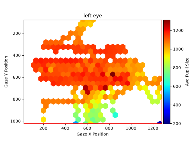
vmin/vmax set the color range, min_samples hides bins with few samples and smooth applies Gaussian smoothing.

plot_pupil_segments(pdf_file=None, interv='1 min', figsize=(15, 5), ylim=None, units='sec', **kwargs)#

Plot the whole dataset chunked up into segments (usually to a PDF file).

Parameters:

pdf_file (Optional[str]) – file name to store the PDF; if None, no PDF is written
interv (float) – duration of each of the segments to be plotted (plain numbers are in units, or with units, e.g. "2 min"); default 1 min
figsize (Tuple[int,int]) – dimensions of the figures
ylim (Tuple[float,float] or None) – y-axis limits for the plots; if None, matplotlib’s automatic limits are used
units (str) – Units of the time axis, passed to plot_pupil(). Default “sec”.
**kwargs – arguments passed to plot_pupil() (e.g., highlight and highlight_color)

Return type:

list of matplotlib.figure.Figure

Returns:

one figure per segment (also returned when pdf_file is given; the figures are then closed)

Examples

Split the 40-second recording into 10-second pieces (one figure each, here only the first is shown):

>>> import pypillometry as pp
>>> from pypillometry import u
>>> import matplotlib.pyplot as plt
>>> d = pp.get_example_data("rlmw_002_short")
>>> d = d.pupil.blinks_detect()
>>> figs = d.plot.plot_pupil_segments(interv=10 * u.sec, units="sec",
...                                   figsize=(10, 3))
>>> for f in figs[1:]:
...     plt.close(f)

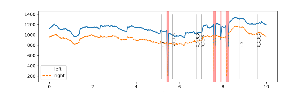
With pdf_file="segments.pdf", the figures are written to a PDF file instead.

plot_scanpath(plot_range=(-inf, inf), eyes=[], show_screen=True, rois=None, roi_style={}, show_onsets=True, title=None, units='sec', ax=None)#

Plot EyeData as a scanpath. Typically used for single trials or another small amount of data. To plot a larger amount of data, use plot_heatmap() instead.

If several eyes are available, they are plotted in the same figure in different colors. You can choose between them using the eyes parameter. The samples are drawn as dots colored by time. The y-axis points down (screen pixel coordinates, as in plot_calibration()).

Parameters:

plot_range (tuple) – The time range to plot (plain numbers are in units, or with units, e.g. (3, 5) * u.min). Default is (-np.inf, +np.inf), i.e. all data.
eyes (list) – The eyes to plot. Default is [], which means all available data (“left”, “right”, average, regression, …)
show_screen (bool) – Whether to plot the screen limits (if an experimental setup is available). Default is True.
rois (List[ROI]) – List of ROIs (ROI) to plot. Default is None.
roi_style (dict) –
Style for the ROIs, passed as keyword arguments to the ROIs’ plot() method. Default is {} (ROI defaults). Example:
```
{
    "facecolor": "red",
    "edgecolor": "black",
    "linewidth": 2,
    "alpha": 0.5
}
```
show_onsets (bool) – Whether to plot the event labels at the gaze position at event onset. Plotted only for the first eye. Default is True.
title (str) – The title of the plot.
units (str) – The units of the time axis and of plain numbers in plot_range (“ms”, “sec”, “min”, “h”). Default “sec”.
ax (matplotlib.axes.Axes, optional) – axes to plot on; default: the current axes

Return type:

matplotlib.axes.Axes

Returns:

the axes of the plot

Raises:

ValueError – if plot_range does not overlap with the data

Examples

Two seconds of gaze of the left eye:

>>> import pypillometry as pp
>>> from pypillometry import u
>>> import matplotlib.pyplot as plt
>>> d = pp.get_example_data("rlmw_002_short")
>>> fig, ax = plt.subplots(figsize=(6, 5))
>>> ax = d.plot.plot_scanpath(plot_range=(10, 12) * u.sec, eyes="left", ax=ax)

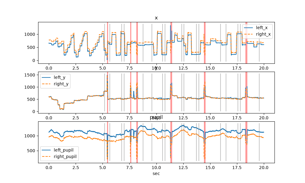
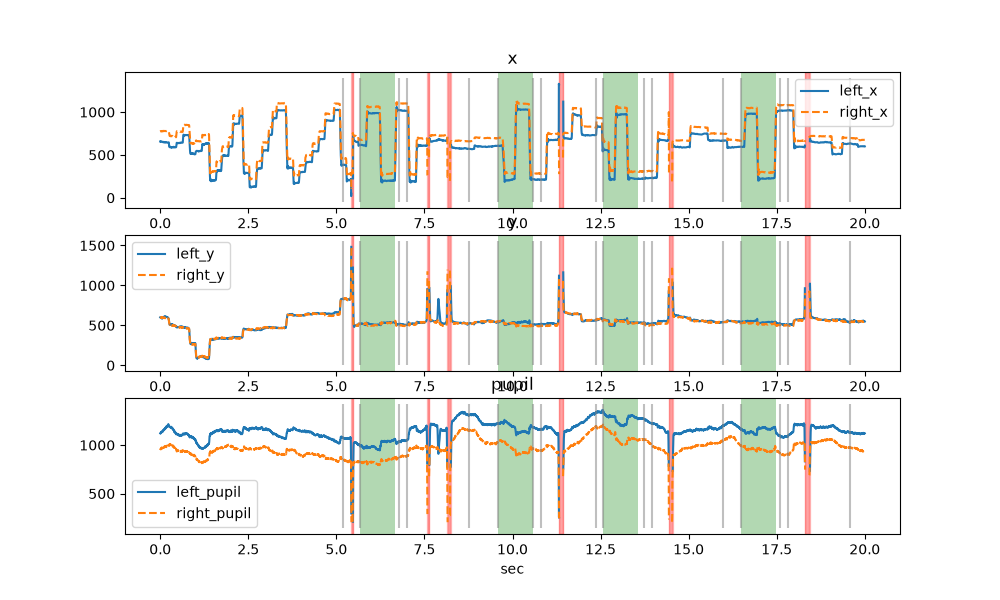
plot_timeseries(plot_range=(-inf, inf), variables=[], eyes=[], units='sec', show_onsets='line', show_masked=True, show_mask_highlight=True, label_prefix='', style=None, highlight=None, highlight_color='lightblue', title=None, axes=None, figsize=None, **kwargs)#

Plot a part of the EyeData. Each variable is plotted in a separate subplot (one below the other), all eyes in the same subplot.

Parameters:

plot_range (tuple) – The time range to plot; plain numbers are in units, values with units are converted (e.g. (0, 20) * u.sec). Default is (-np.inf, +np.inf), i.e. all data.
variables (list) – The data to plot. Default is [], which means all available data will be plotted. Available data are [“x”,”y”,”pupil”] but can be extended by the user.
eyes (list) – The eyes to plot. Default is [], which means all available data (“left”, “right”, “average”, “regression”, …)
units (str) – The units of the time axis and of plain numbers in plot_range (“ms”, “sec”, “min”, “h”). Default “sec”.
show_onsets (str) – Whether to plot markers for the event onsets. One of “line” (vertical lines), “label” (text label), “both” (both lines and labels), or “none” (no markers). Default is “line”.
show_masked (bool) – Whether to plot the data in masked regions. If True (default), plots all data including masked regions. If False, masked data points are not plotted (gaps in the line).
show_mask_highlight (bool) – Whether to highlight masked regions (default mask policy: interpolated samples are not masked) with a light red background. Default is True.
label_prefix (str) – Prefix to add to labels in the legend. Useful for overlaying multiple datasets. Default is “” (no prefix).
style (dict) –
Styling for plotted lines. Can be:
- Single dict: Applied to all eyes with automatic differentiation (e.g., {‘color’: ‘red’})
- Dict of dicts: Per-eye styling (e.g., {‘left’: {‘linestyle’: ‘-‘}, ‘right’: {‘linestyle’: ‘–‘}})
Default is None (uses matplotlib defaults with automatic per-eye colors and linestyles).
highlight (Intervals, Epochs or list of them, optional) – periods to shade in the background (e.g., trials from get_intervals()), converted to the units of the time axis
highlight_color (color or list of colors, optional) – color of the shading: one for all or one per element of highlight; default “lightblue”
title (str) – title of the figure
axes (list of matplotlib.axes.Axes, optional) – axes to plot on, one per variable (e.g., fig.axes of an earlier call, to overlay several datasets); default: a new figure
figsize (tuple) – size of the new figure
**kwargs – passed to matplotlib.axes.Axes.plot() for all lines (after style)

Return type:

matplotlib.figure.Figure

Returns:

the figure of the plot

Raises:

ValueError – if show_onsets is not one of the allowed values, if plot_range does not overlap with the data or if axes does not contain one axes per variable

Examples

>>> import pypillometry as pp
>>> from pypillometry import u
>>> import matplotlib.pyplot as plt
>>> d = pp.get_example_data("rlmw_002_short")
>>> fig = d.plot.plot_timeseries(plot_range=(0, 20) * u.sec, units="sec",
...                              figsize=(10, 6))

The first second after each stimulus, shaded in all subplots:

>>> import pypillometry as pp
>>> from pypillometry import u
>>> import matplotlib.pyplot as plt
>>> d = pp.get_example_data("rlmw_002_short")
>>> fig = d.plot.plot_timeseries(plot_range=(0, 20) * u.sec, figsize=(10, 6),
...                              highlight=d.get_epochs("S_", (0, 1000) * u.ms),
...                              highlight_color="green")

plot_timeseries_segments(pdf_file=None, interv='1 min', figsize=(15, 5), ylim=None, eyes=[], variables=[], units='sec', **kwargs)#

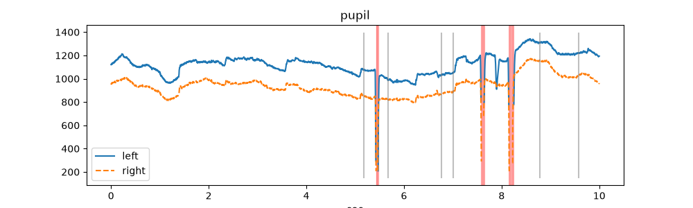
Plot the whole dataset chunked up into segments (usually to a PDF file).

Parameters:

pdf_file (str) – file name to store the PDF; if None, no PDF is written
interv (float) – duration of each of the segments to be plotted (plain numbers are in units, or with units, e.g. 10 * u.sec); default 1 min
figsize (Tuple[int,int]) – dimensions of the figures
ylim (Tuple[float,float] or None) – y-axis limits for all subplots
eyes (list) – list of eyes to plot; if empty, all available eyes are plotted
variables (list) – list of variables to plot; if empty, all available variables are plotted
units (str) – units for the time axis (and plain numbers in interv); default “sec”
**kwargs – additional arguments passed to plot_timeseries() (e.g., highlight and highlight_color)

Return type:

list of matplotlib.figure.Figure

Returns:

one figure per segment (also returned when pdf_file is given; the figures are then closed)

Examples

Split the 40-second recording into 10-second pieces (one figure each, here only the first is shown):

>>> import pypillometry as pp
>>> from pypillometry import u
>>> import matplotlib.pyplot as plt
>>> d = pp.get_example_data("rlmw_002_short")
>>> figs = d.plot.plot_timeseries_segments(interv=10 * u.sec, units="sec",
...                                        variables="pupil", figsize=(10, 3))
>>> for f in figs[1:]:
...     plt.close(f)

With pdf_file="segments.pdf", the figures are written to a PDF file instead.

WARN_SEGMENTS = 500#: a *_segments plot with more figures than this warns

Plotting (d.plot)#

Time series#

Blinks, masks and intervals#

Gaze#

Experimental setup and foreshortening#

All plots#

Plotting (`d.plot`)#