Working with the results

rmedsem() returns an object of class rmedsem. Besides printing it, there are several functions to summarize the results, extract estimates for further processing, and visualize them. We use the simple mediation model from the Getting started section as an example:

library(rmedsem)

mod.txt <- "
  read ~ math
  science ~ read + math
"
mod <- lavaan::sem(mod.txt, data = hsbdemo)
out <- rmedsem(mod, indep = "math", med = "read", dep = "science")

Detailed output and compact summary

Printing the object gives a detailed, step-by-step description of the tests of the indirect effect and of the Baron & Kenny and Zhao, Lynch & Chen approaches:

out
#> Significance testing of indirect effect (standardized)
#> Model estimated with package 'lavaan'
#> Mediation effect: 'math' -> 'read' -> 'science'
#> 
#>                          Sobel          Delta    Monte-Carlo
#> Indirect effect          0.251          0.251          0.251
#> Std. Err.                0.046          0.046          0.047
#> z-value                  5.501          5.446          5.374
#> p-value               3.79e-08       5.15e-08       7.71e-08
#> CI              [0.161, 0.340] [0.160, 0.341] [0.160, 0.343]
#> 
#> Baron and Kenny approach to testing mediation
#>    STEP 1 - 'math' -> 'read' (X -> M) with B=0.662 and p<0.001
#>    STEP 2 - 'read' -> 'science' (M -> Y) with B=0.378 and p<0.001
#>    STEP 3 - 'math' -> 'science' (X -> Y) with B=0.380 and p<0.001
#>             As STEP 1, STEP 2 and STEP 3 as well as the Sobel's test above
#>             are significant the mediation is partial.
#> 
#> Zhao, Lynch & Chen's approach to testing mediation
#> Based on p-value estimated using Monte-Carlo
#>   STEP 1 - 'math' -> 'science' (X -> Y) with B=0.380 and p<0.001
#>             As the Monte-Carlo test above is significant, STEP 1 is
#>             significant and their coefficients point in same direction,
#>             there is complementary mediation (partial mediation).
#> 
#> Effect sizes
#>    RIT = (Indirect effect / Total effect)
#>          (0.251/0.631) = 0.397
#>          Meaning that about 40% of the effect of 'math'
#>          on 'science' is mediated by 'read'
#>    RID = (Indirect effect / Direct effect)
#>          (0.251/0.380) = 0.659
#>          That is, the mediated effect is about 0.7 times as
#>          large as the direct effect of 'math' on 'science'
#>    Upsilon (v) = Variance in Y explained indirectly by X through M
#>          v(unadj) = 0.063, v(adj) = 0.061

summary() condenses the same results into a table of the indirect (for each estimation method), direct and total effects, the resulting type of mediation and the effect sizes:

s <- summary(out)
s
#> Mediation analysis: 'math' -> 'read' -> 'science'
#> Estimated with 'lavaan' (standardized), N = 200
#> 
#> Effects (95% CI):
#>                        Estimate Std. Err. z-value  p-value Lower Upper
#> Indirect (Sobel)          0.251     0.046   5.501 3.79e-08 0.161 0.340
#> Indirect (Delta)          0.251     0.046   5.446 5.15e-08 0.160 0.341
#> Indirect (Monte-Carlo)    0.251     0.047   5.374 7.71e-08 0.160 0.343
#> Direct                    0.380     0.065         4.43e-09 0.253 0.507
#> Total                     0.631     0.037                  0.559 0.703
#> 
#> Type of mediation (significant: p < 0.05):
#>   Baron & Kenny:      partial mediation
#>   Zhao, Lynch & Chen: complementary mediation (partial mediation)
#>                       (based on Monte-Carlo test)
#> 
#> Effect sizes:
#>   RIT = 0.397
#>   RID = 0.659
#>   Upsilon = 0.061
#>   Upsilon (unadj.) = 0.063

The summary is itself an object whose elements can be used in further analyses, e.g., the type of mediation or the table of effects:

s$mediation
#> $bk
#> [1] "partial"
#> 
#> $zlc
#> [1] "complementary"
s$effects
#>     effect method  estimate         se     zval         pval     lower
#> 1 indirect  sobel 0.2506159 0.04556196 5.500552 3.786031e-08 0.1613161
#> 2 indirect  delta 0.2506159 0.04601847 5.445986 5.151917e-08 0.1604214
#> 3 indirect  montc 0.2506159 0.04669944 5.373859 7.706911e-08 0.1602372
#> 4   direct   <NA> 0.3801172 0.06478771       NA 4.434311e-09 0.2531357
#> 5    total   <NA> 0.6309719 0.03730960       NA           NA 0.5588379
#>       upper
#> 1 0.3399157
#> 2 0.3408105
#> 3 0.3433785
#> 4 0.5070988
#> 5 0.7028962

Extracting estimates

The standard extractor functions coef(), confint() and nobs() work for rmedsem objects:

coef(out)
#>  indirect    direct     total 
#> 0.2506159 0.3801172 0.6309719
confint(out)
#>              2.5 %    97.5 %
#> indirect 0.1602372 0.3433785
#> direct   0.2531357 0.5070988
#> total    0.5588379 0.7028962
nobs(out)
#> [1] 200

The indirect effect is estimated with several methods (here Sobel, Delta and Monte-Carlo). They share the same point estimate but differ in their standard errors and intervals. By default, coef() and confint() use the method that also underlies the Zhao, Lynch & Chen approach (Monte-Carlo for lavaan and modsem, bootstrap for cSEM, and the posterior for blavaan). Use the method argument to choose a different one:

confint(out, parm = "indirect", method = "sobel")
#>              2.5 %    97.5 %
#> indirect 0.1613161 0.3399157

The level of all intervals is set when calling rmedsem() with the ci.two.tailed argument:

out90 <- rmedsem(mod, indep = "math", med = "read", dep = "science",
                 ci.two.tailed = 0.90)
confint(out90)
#>                5 %      95 %
#> indirect 0.1749096 0.3287469
#> direct   0.2735509 0.4866835
#> total    0.5674115 0.6933806

as.data.frame() returns the estimates of the indirect effect for all methods as a data frame:

as.data.frame(out)
#>   package method      coef         se     zval         pval     lower     upper
#> 1  lavaan  sobel 0.2506159 0.04556196 5.500552 3.786031e-08 0.1613161 0.3399157
#> 2  lavaan  delta 0.2506159 0.04601847 5.445986 5.151917e-08 0.1604214 0.3408105
#> 3  lavaan  montc 0.2506159 0.04669944 5.373859 7.706911e-08 0.1602372 0.3433785

Effect sizes

The effect sizes are available through dedicated functions:

RIT(out)      # ratio of indirect to total effect
#> [1] 0.3973407
RID(out)      # ratio of indirect to direct effect
#> [1] 0.6593122
Upsilon(out)  # variance in 'science' explained indirectly by 'math' via 'read'
#> [1] 0.06073778
Upsilon(out, adjusted = FALSE)
#> [1] 0.06280834

Plots

plot() shows a coefficient plot of the indirect (for each method), direct and total effects, or a pie chart of the indirect and direct effects:

plot(out)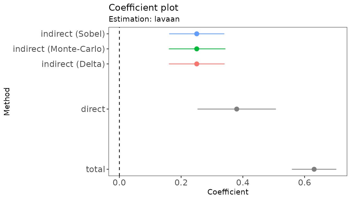

plot(out, type = "effect")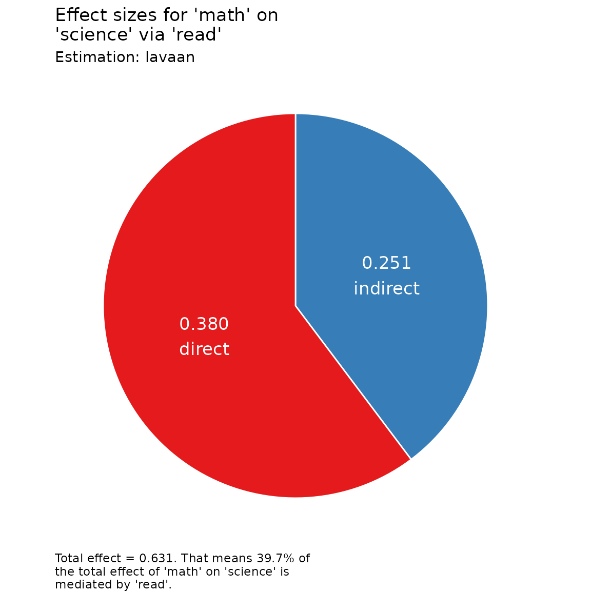

Bayesian models: equal-tailed intervals or HDI

For models estimated with blavaan, the intervals are credible intervals computed from the posterior samples. By default, these are equal-tailed intervals (the 2.5% and 97.5% quantiles for ci.two.tailed = 0.95). Set hdi = TRUE to obtain highest density intervals (HDI) instead, which requires the HDInterval package:

library(blavaan)
bmod <- bsem(mod.txt, data = hsbdemo, n.chains = 3, burnin = 500, sample = 500,
             seed = 1, bcontrol = list(cores = 3, refresh = 0))

out.ci  <- rmedsem(bmod, indep = "math", med = "read", dep = "science")
out.hdi <- rmedsem(bmod, indep = "math", med = "read", dep = "science",
                   hdi = TRUE)

confint(out.ci)
#>              2.5 %    97.5 %
#> indirect 0.1573832 0.3398089
#> direct   0.2428480 0.5059463
#> total    0.5425477 0.6988324
confint(out.hdi)
#>              lower     upper
#> indirect 0.1591007 0.3412056
#> direct   0.2464126 0.5102203
#> total    0.5507015 0.7025515
summary(out.hdi)
#> Mediation analysis: 'math' -> 'read' -> 'science'
#> Estimated with 'blavaan' (standardized), N = 200
#> 
#> Effects (95% HDI):
#>                  Estimate Std. Err. z-value p-value Lower Upper
#> Indirect (Bayes)    0.248     0.046   5.359   0.000 0.159 0.341
#> Direct              0.380     0.067           0.000 0.246 0.510
#> Total               0.629     0.039                 0.551 0.703
#> For Bayesian estimates, 'p-value' is the posterior probability of
#> the opposite sign.
#> 
#> 
#> Effect sizes:
#>   RIT = 0.395
#>   RID = 0.653
#>   Upsilon = 0.060
#>   Upsilon (unadj.) = 0.062